Previous page : Data analysis, part 2, more linear Data
Next page : Analysis 4, errors on both variables
Non-linear data
In the following, we have yet again done some measurement of how some physical quantity B depends on some other physical quantity A. (The data and practical analysis can be found in the file analysis3. xlsx.) We will look at two ways to do it: either linearizing it using logarithms or if that fails, using a bit of trial and error.
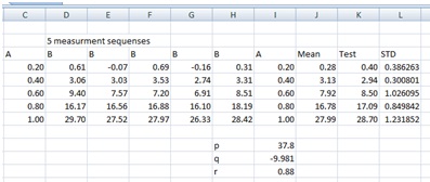
The data is in the file analysis3 V2 non linear data.
We have the following:

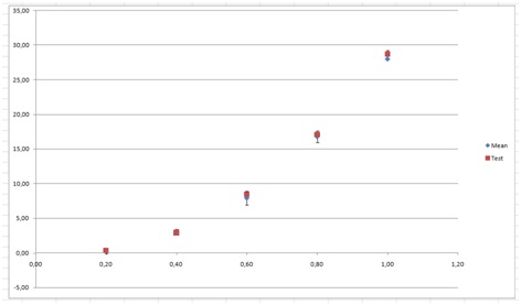
If we plot the mean of B against A we get:
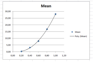
This is clearly not linear. We could now try to add a trend line, or do the “log thingy”. An exponential trend line does not fit very well, but a quadratic polynomial does, with an R2 of 0.999.
About the “log thingy”
(The name “the log thingy” for using logarithms for linearization was given by a student of mine Carin (thanks Karin).)
Suppose we have data that first an exponential function, B=c·aA then if we take the logarithm on both sides (I have chosen logarithms with the base 10) we get
lg B=lg c + A lg a
A plot of lg B vs. A would now be a straight line since the equation above is in the form “y=mx+c”. The slope will be lg a and the “y”-intercept will be lg c. Trying this would yield:
 Clearly not linear.
Now assume we have a power function in the form B=c·An . Yet again we do the log trick.
lg B=lg c + n lg A
Now, if we would plot lg B vs. lg A we would expect to get a straight line with the slope n and the “y”-intercept” lg c . Trying this gets us:
 This does indeed look linear, as can be seen even better after adding a trend line.
Analysing non-linear data
So, we have found out that it can be an exponential relation. The problem now is to find the uncertainties. We cannot use the errors in our data directly since we do some mathematical operation on them that changes their values. In the case of a power function, it is much easier since we only need to multiply the errors by lg A because we have
lg B=lg c + A lg a.
In that case, we only need to make a new error column by multiplying the old error (STD or SEM) by lg A.
In the case of an exponential relation, it becomes somewhat more complicated since we change the values by doing some non-linear operation on them (the logarithm). What we can do is calculate the lower and upper values of the values including the errors. I.e. we make new tables with the values of B plus the errors in B and B minus the errors in B.
 Have a look in the Excel file, in the leaf called Analysis Part 2, and click on a cell if you are unsure of what is done. Next, we take the logarithm of the values. Any negative values will cause problems, but we can fix that later on. We get:
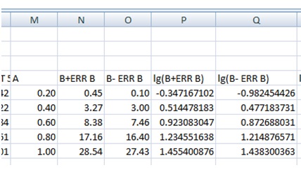
For each mean A we now have a pair of points, a lower and an upper. The average (sum / 2) will be our new value, and the difference divided by 2 is our new error in lg B. For the point where we don’t have a lower value, we keep lg B of our average as our lg B , and the difference between that and the upper value as our error in. In this case, we don’t have any such points though.
 We get:
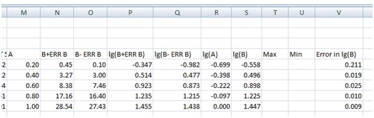
Plotting lg B vs. lg A, with the error bars from column S, will now give us:
 The error bars are very small, except for the smallest value of B, since the taking logarithm gives us the relative errors rather than the absolute errors.
Since the error bars are so small one might try the trick of first subtracting the trend line values. I will though try to fit a line directly. To facilitate this I first enlarge the graph as much as possible.
We can now proceed as in Data analysis 2. We add two columns for our min and maximum slope, and then we try to make the lines fit the data.
 This gives us the following graphs:
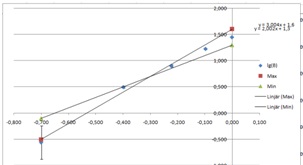
Enlarge the graph as much as possible then start to tweak the values in columns T and U. As we can see we have a problem going through the lowermost point. We may either enlarge all error bars, or possibly just this one, but we have to argue for our choice in our work. In this case, we might argue that we might actually have some error in the measurement of the length and that this will influence the error in the shortest distance. After a few minutes I found this:
 This gave me the graph:
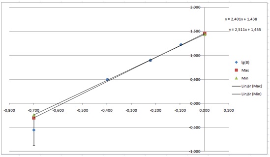
One line will here miss the lower error bar, and another the error bars of the second point, but not by much.
From this, we can find the max and minimum values of the slope, i.e. the power of our power function. We have 2.401 and 2.511. The average of this will be our power, and half the difference will be our error. We get 2.456 and 0.055, so we get n=2.4±0.1, after rounding our values.
Next, we look at the “y”-intercept, which will be the logarithm of the coefficient in of the power function, i.e. lg c of the c in B=c·An . We have 1.438 and 1.455. Ten to the power of those values gives us 27.163 and 28.51. This gives us the mean 27.96 and the error 0.54, i.e. . c=28±1.
If we put this together we get
B=(28±1)·A2.4±0.1
Not too bad, considering that I used the formula
=$C47^((RAND()*2-1)*0.4+2.5)*(27+(RAND()*2-1)*2.4)+(RAND()*2-1)*0.5
I.e. the data was randomly chosen with a coefficient of 27±2.4 and an exponent of 2.5±0.4.
Also, seeing something like I would guess we are actually having an exponent of 2.5, since exponents in physics are mostly multiples of 1/2, or in rare cases, multiples of 1/3.
Using the line of best-fit tool and trial and error
Now, suppose we were not able to do the above. We could then try to use the line of best-fit tool. We first plot the data, with error bars, and fit a line of best fit. In this, a quadratic would fit the best (R2=0.999), but that would give us an equation of the form
B=38.3A2–11.5A+1.4
Unless we have a particular reason to expect something like this (for example if we don’t start at the say time 0, velocity 0, or something similar) then this would be a highly unusual equation. Anyhow, let us though work with this for a while. I would add places in Excel for the coefficients of the quadratics. Say we have
B=pA2 + qA + r
Then we make a new column, calculating the values according to the above equation. In the file, I have called that column “Test”.
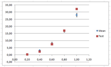
The graph of Mean and Test vs. A would look like this:
Then we start to tweak the variables, one by one to see the possible ranges so that the points are still within the error bounds. Starting with p we seem to be able to use values between 37.1 and 37.9. Keeping the latter I start with tweaking q. I got that values between –10.2 and –9.7 seems to work. Finally, I try with the coefficient r. The range here seems to be from about 0.5 to 1.1. Trying with q=–10.2 and p=0.9 we can extend the range of p up to 38.3 But using that we can lower q to –11.5, and using that we can increase r to 1.4. Stopping here we have that

The values are highly uncertain though, so I would choose to have the ranges

or
B=(38±1)A2–(10±2)B+1±1
This is better than anything, but we should also be aware of that this is just a fit to the data points we have, without any theoretical reason why it should be this particular equation. That is true for the previous solution too, but it is more likely we could connect that to some kind of theory.
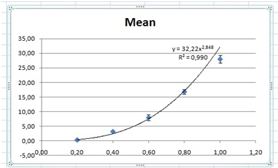
We could try using Excel’s ability to fit a power function. This gives us
B=32.22·A2.848
Here the trend line clearly misses the last point’s error bar.
We now create places for the variables c and n, and then add a column for calculating the corresponding function values.
 We then plot a new graph, including the new column.
We then start to tweak the values of the variables c and n.
After some tweaking, I found that c=26.5 and n=2.3 seem to work, and on the other end of the scale that c=29.0 and n=2.7.
This would give us an average of c of 27.5 with an error of 1.25, i.e. 28±2 and for n, 2.5±0.2, which is almost exactly the same as with the previous method.
Previous page : Data analysis, part 2, more linear Data
Next page : Analysis 4, errors on both variables