Hyperbolic functions – The cosinus hyperbolicus and its inverse

Up a level : The hyperbolic functions
Next page : The sinus hyperbolicus function

The hyperbolic functions can be used to solve integrals, among other things, but what are the hyperbolic functions? To get to that we will first redefine our concept of the circular angle.

We will define the circular angle as the area of a unit circular sector with a central angle of 2θ.

The area will now be

$A = \frac{{2\theta }}{{2\pi r}}\pi {r^2} = \theta ,\quad r = 1$

Then we define cos of the angle as the height of the triangle, that is the distance from the origin to the middle of the side opposing the central angle, and we will define the sine of the angle as half of the length of the base, where the base is the opposing the central angle. If the sector is placed as in the figure above.

By these definitions cos and sine will keep their meaning, even if the definition of the angle has changed. So, what to do now? The equation of a circle is

${x^2} + {y^2} = 1$

Now let us look at

${x^2} - {y^2} = 1$

$y = \pm \sqrt {{x^2} - 1}$

and do as above with the circle. The equation describes a pair of hyperbolae. We will thus define the hyperbolic angle as the area of the hyperbolic sector as shown in the figure.

Next, we define two functions, sinus hyperbolicus, sinh θ and cosinus hyperbolicus, cosh θ, in an analogous manner as for the circular functions.

Ok, this is nifty and fine. But how to calculate these two new functions? It is actually easier to find the inverse functions. We will try to find a function that gives us the x-coordinate of the point Q, given the red area, θ, in the figure below.

We will do this by finding the grey area by integration, then subtracting that from the triangle formed by the origin and the points P and Q.

So, for the grey area, we get

$2\int\limits_1^x {\sqrt {{x^2} - 1} \;dx}$

We can use the result from this page where we found that

$\begin{gathered} 2\int {\sqrt {{x^2} - 1} \,dx = } \hfill \\ \quad = 2\left( {\frac{1}{2}x\sqrt {{x^2} - 1} - \frac{1}{2}\ln \left( {x + \sqrt {{x^2} - 1} } \right)} \right) + C \hfill \\ \quad = x\sqrt {{x^2} - 1} - \ln \left( {x + \sqrt {{x^2} - 1} } \right) + C \hfill \\ \end{gathered}$

To get

$\begin{gathered} 2\int\limits_1^x {\sqrt {{x^2} - 1} \;dx} = \left[ {x\sqrt {{x^2} - 1} - \ln \left( {x + \sqrt {{x^2} - 1} } \right)} \right]_1^x \hfill \\ \quad = x\sqrt {{x^2} - 1} - \ln \left( {x + \sqrt {{x^2} - 1} } \right) \hfill \\ \quad \;\; - \left( {1\sqrt {{1^2} - 1} - \ln \left( {1 + \sqrt {{1^2} - 1} } \right)} \right) \hfill \\ \quad = x\sqrt {{x^2} - 1} - \ln \left( {x + \sqrt {{x^2} - 1} } \right) \hfill \\ \end{gathered}$

The rectangular area OPQ is

$\frac{{x \cdot 2y}}{2} = xy = x\sqrt {{x^2} - 1}$

Now subtracting the grey area from the above gives us the red area

$\begin{gathered} \theta = x\sqrt {{x^2} - 1} - \left( {x\sqrt {{x^2} - 1} - \ln \left( {x + \sqrt {{x^2} - 1} } \right)} \right) \hfill \\ \quad = \ln \left( {x + \sqrt {{x^2} - 1} } \right) \hfill \\ \end{gathered}$

This will give us the following graph.

I have also added a negative branch if we would allow us to have negative hyperbolic angles.

The cosinus hyperbolicus function

Now to the function we are looking for. We wanted a function that gives us the x-coordinate of the point Q given the hyperbolic angle, i.e. the inverse of the function we just found.

$\theta = \ln \left( {x + \sqrt {{x^2} - 1} } \right)$

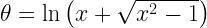
Starting with taking the natural logarithm of both sides we get

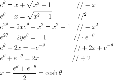
$\begin{gathered} {e^\theta } = x + \sqrt {{x^2} - 1} \quad \quad \quad \quad // - x \hfill \\ {e^\theta } - x = \sqrt {{x^2} - 1} \quad \quad \quad \quad /{/^2} \hfill \\ {e^{2\theta }} - 2x{e^\theta } + {x^2} = {x^2} - 1\quad // - {x^2} \hfill \\ {e^{2\theta }} - 2y{e^\theta } = - 1\quad \quad \quad \quad \;// \cdot {e^{ - \theta }} \hfill \\ {e^\theta } - 2x = - {e^{ - \theta }}\quad \quad \quad \quad \;\;// + 2x + {e^{ - \theta }} \hfill \\ {e^\theta } + {e^{ - \theta }} = 2x\quad \quad \quad \quad \;\;\;\;// \div 2 \hfill \\ x = \frac{{{e^\theta } + {e^{ - \theta }}}}{2} = \cosh \theta \hfill \\ \end{gathered}$

This function, the cosinus hyperbolicus is thus the average of the exponential function and its reflection in the y-axis. Below we can see a graph of this function.

As the cos function, it has an y-intercept at (0,1). We can also compare it with the expression

$\cos (\theta ) = \frac{{{e^{i\theta }} + {e^{ - i\theta }}}}{2}$

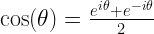
found here. The difference is thus the imaginary unit used in the exponents in the hyperbolic function.

The inverse function

This above function has several interesting properties as we will see. We have already found its inverse.

$\theta = {\text{arcosh }}x = {\cosh ^{ - 1}}x = \ln \left( {x + \sqrt {{x^2} - 1} } \right)$

This is the arcose hyperbolicus function. It is called “ar” not “arc”. The reason for this is that the arccos-function gives something that can be seen as corresponding to an arc length, whilst the arcosh gives us an area.

Up a level : The hyperbolic functions
Next page : The sinus hyperbolicus function

Last modified: Dec 28, 2023 @ 14:07