Mclaurin series - a first take

Up a level : Power Series
Previous page : Power Series - an introduction
Next page : Taylor series

A polynomial of degree n can perfectly fit through n-1 points (not above each other) so maybe an infinite degree polynomial could fit infinitely many points along a continuous function?

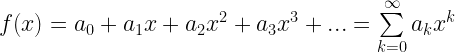
Let us say we have some function f (x) and we want to express it as a power series as

$f(x) = {a_0} + {a_1}x + {a_2}{x^2} + {a_3}{x^3} + ... = \sum\limits_{k = 0}^\infty {{a_k}{x^k}}$

To retrieve the constants we can first set x=0. This will give us

$f(0) = {a_0}$

Next, we differentiate our function to get

$f'(x) = {a_1} + 2{a_2}x + 3{a_3}{x^2} + 4{a_4}{x^3} + ... = \sum\limits_{k = 0}^\infty {k{a_k}{x^{k - 1}}}$

This gives us

$f'(0) = {a_1}$

We repeat with the second derivative to get

$f''(x) = 2{a_2} + 3 \cdot 2{a_3}x + 4 \cdot 3{a_4}{x^2} + ... = \sum\limits_{k = 0}^\infty {k(k - 1){a_k}{x^{k - 2}}}$

This gives us

$f''(0) = 2{a_2}\quad \Rightarrow {a_2} = \frac{{f''(0)}}{2}$

We repeat this to get

${a_3} = \frac{{{f^{(3)}}(0)}}{{3!}},\quad {a_4} = \frac{{{f^{(4)}}(0)}}{{4!}},\quad ...$

All and all we get

$f(x) = \sum\limits_{k = 0}^\infty {\frac{{{f^{(k)}}(0)}}{{k!}}{x^k}}$

This is the Mclaurin series expansion. This is often called just the series expansion or Mclauritn expansion of the function. It is also often called a Taylor expansion of the function, since, as we will see on the next page, Mclauritn expansions are just a special case of the Taylor expansion. In the following pages, I will mainly call them Taylor expansions or series expansions.

As we saw on the previous page we might not have an equality all for all values of x, and this we shall examine after a few examples.

A first few Examples

Let us start with something we already know

$f(x) = \frac{1}{{1 - x}} = {(1 - x)^{ - 1}}$

Is useful is to make a table of derivatives, and the corresponding values when x=0.

k	f ^(k)(x)	f ^(k)(0)
0	${(1 - x)^{ - 1}}$	0!
1	$1 \cdot {(1 - x)^{ - 2}}$	1!
2	$1 \cdot 2 \cdot {(1 - x)^{ - 3}}$	2!
3	$1 \cdot 2 \cdot 3 \cdot {(1 - x)^{ - 4}}$	3!
4	…	…

(Observe that the 0^th derivative is the same as doing nothing.)

This gives us

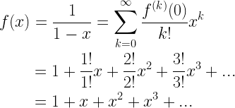
$\begin{gathered} f(x) = \frac{1}{{1 - x}} = \sum\limits_{k = 0}^\infty {\frac{{{f^{(k)}}(0)}}{{k!}}{x^k}} \hfill \\ \quad \quad \; = 1 + \frac{{1!}}{{1!}}x + \frac{{2!}}{{2!}}{x^2} + \frac{{3!}}{{3!}}{x^3} + ... \hfill \\ \quad \quad \; = 1 + x + {x^2} + {x^3} + ... \hfill \\ \end{gathered}$

as expected. We shall look at what values this is true for later on. As you may verify we also have

$\frac{1}{{1 + x}} = 1 - x + {x^2} - {x^3} + ...$

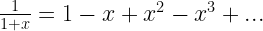
This you can do by either doing the series expansion using the derivatives or by just substituting –x for x in the above expansion.

The exponential function, e^x

This is probably the most well-known. Since the successive derivatives of e^x are all e^x and e⁰=1 we get that

k	f ^(k)(x)	f ^(k)(0)
0	e^x	1
1	e^x	1
2	e^x	1
3	e^x	1
4	…	…

This gives us

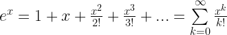
${e^x} = 1 + x + \frac{{{x^2}}}{{2!}} + \frac{{{x^3}}}{{3!}} + ... = \sum\limits_{k = 0}^\infty {\frac{{{x^k}}}{{k!}}}$

This converges very fast if |x|<1 since the factorial function grows so fast. In the graph below e^x and the first few terms of the series expansion is graphed.

One can see that the more terms we add, the closer to e^x we get. We can also see that it sways back and forth widely when x is negative. At this scale the graph of the series with 30 terms would be indistinguishable from the graph of e^x.

The sine and cos functions

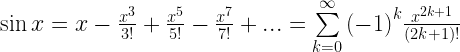
To start with, for this to work, x must be in radians.

Our table of derivatives will now be

k	f ^(k)(x)	f ^(k)(0)
0	sin x	0
1	cos x	1
2	–sin x	0
3	–cos x	–1
4	sin x	0
5	…	…

As we can see, the pattern will then repeat.

This gives us

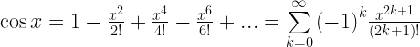
$\sin x = x - \frac{{{x^3}}}{{3!}} + \frac{{{x^5}}}{{5!}} - \frac{{{x^7}}}{{7!}} + ... = \sum\limits_{k = 0}^\infty {{{( - 1)}^k}\frac{{{x^{2k + 1}}}}{{(2k + 1)!}}}$

To get the series expansion of the cos function we may just start at the second row in the table to get

$\cos x = 1 - \frac{{{x^2}}}{{2!}} + \frac{{{x^4}}}{{4!}} - \frac{{{x^6}}}{{6!}} + ... = \sum\limits_{k = 0}^\infty {{{( - 1)}^k}\frac{{{x^{2k + 1}}}}{{(2k + 1)!}}}$

A practical use

The above series are often used in computers to calculate the mentioned functions – either in software or in hardware. The values of x is scaled first though.

Say we need to calculate e^21.4. We start with the fact that e^21.4 = e²¹ e^0.4.

To calculate e²¹ we calculate e², e⁴, e⁸ and e¹⁶ by successive squaring. Then since e²¹= e¹⁶e⁴ e we only need to multiply those numbers. That would give us six multiplications (instead of 20). This would give us 1318815734.48321 calculated with 15 significant figures (accentually with 64 bit floating point numbers).

Then we calculate e^0.4 using the series above.

k	series up to k
0	1.00000000000000
1	1.40000000000000
2	1.48000000000000
3	1.49066666666667
4	1.49173333333333
5	1.49181866666667
6	1.49182435555556
7	1.49182468063492
8	1.49182469688889
9	1.49182469761129
10	1.49182469764018
11	1.49182469764123
12	1.49182469764127
13	1.49182469764127
14	1.49182469764127

As you can see the value does not change after the 12^th term. Finally, multiplying these results together gives us e^21.4≈1967441884.33997.

Similarly, we scale the angles to the first quadrant (or actually, even to the first octant) since all the values of cos and sine can be rescaled to that interval. We have for example that

$\begin{gathered} \sin (410^\circ ) = \sin (410^\circ - 360^\circ ) \hfill \\ \quad = \sin (50^\circ ) = \cos (90^\circ - 50^\circ ) \hfill \\ \quad = \cos (40^\circ ) = \cos \left( {\frac{{2\pi }}{9}} \right) \hfill \\ \end{gathered}$

Using the series for cos we get that already after 9 terms (k=16) the value does not change any more, so this ought to be a good approximation of sin(410°).

Up a level : Power Series
Previous page : Power Series - an introduction
Next page : Taylor series

Last modified: Dec 27, 2023 @ 22:44