The fundamental theorem of calculus

Up a level : Integrals
Previous page : Integrals - a definition - Riemann Integrals
Next page : The connection between the definite and indefinite integral

Antiderivatives

For the next step, we need to be able to work out the inverse of derivatives. I.e. given a function, we need to find what other function would have the first function as its derivative. We call that function the antiderivative or the primitive function of the first function and we denote it by using the capital letter corresponding to the lowercase letter for the original function.

An antiderivative, or primitive function of f (x) is thus written as F(x).

Examples

Since the derivative of x² is 2x an antiderivative of 2x is x². Why I write “an” and not “the” is because all functions of the form x²+C, where C is a constant will have the same derivative. We thus have that if f (x) = 2x, then F(x)= x²+C. You can always verify that you have found an antiderivative by taking the derivative of what you got. If it is correct then you should get your original function back.

You can thus easily verify that the following rule is correct.

$f(x) = {x^n} \Rightarrow F(x) = \frac{{{x^{n + 1}}}}{{n + 1}} + C$

Since we (hopefully) know quite many differentiation rules then we almost automatically know a lot of antiderivative rules. We can just use our table backwards.

Now to the main star of this section:

The fundamental theorem of calculus

Yet again, we shall look at the area between the function, the x-axis and the lines x=a and x=b. Let us also just call the end value x. For different values of x, the area will be different. The area will thus be a function of the value of x. We have

$A = A(x)$

If x changes by a small value Δx the area will change by a value ΔA. In the figure, ΔA is the orange + the gray area. We have that

$\Delta A = f(x)\Delta x + \varepsilon$

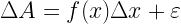
where epsilon is the error, and also the grey area. Now, let us divide by Δx. We get

$\frac{{\Delta A}}{{\Delta x}} = f(x) + \frac{\varepsilon }{{\Delta x}}$

That means that

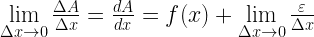
$\mathop {\lim }\limits_{\Delta x \to 0} \frac{{\Delta A}}{{\Delta x}} = \frac{{dA}}{{dx}} = f(x) + \mathop {\lim }\limits_{\Delta x \to 0} \frac{\varepsilon }{{\Delta x}}$

We know that

$\left| \varepsilon \right| \leqslant \left| {\Delta y\Delta x} \right| = \left| {(f(x + \Delta x) - f(x))\Delta x} \right|$

since the triangular-shaped grey area is less than a rectangle with the same base and height. So

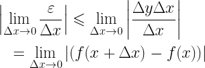
$\begin{gathered} \left| {\mathop {\lim }\limits_{\Delta x \to 0} \frac{\varepsilon }{{\Delta x}}} \right| \leqslant \mathop {\lim }\limits_{\Delta x \to 0} \left| {\frac{{\Delta y\Delta x}}{{\Delta x}}} \right| \hfill \\ \quad = \mathop {\lim }\limits_{\Delta x \to 0} \left| {(f(x + \Delta x) - f(x))} \right| \hfill \\ \end{gathered}$

This means that

$\frac{{dA}}{{dx}} = f(x)$

But if we know the derivative of a function, then we could find the antiderivative to find the original function – and that means that we should be able to find the area function by taking the antiderivative of f (x). We get

$A(x) = F(x) + C$

We know that for x=a the area is 0 so we get

$A(a) = F(a) + C = 0$

and thus

$C = - F(a)$

For x=b we get

$A(b) = F(b) + C = F(b) - F(a)$

But this is exactly what we get from the Riemann integral defined in the previous page. This will finally give us the fundamental theorem of calculus

$\int\limits_a^b {f(x)dx = F(b) - F(a)}$

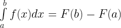
We can in other words find the integral, the limit of the sum of ever smaller rectangles under a function by finding the antiderivative of the function.

In practice we often write the theorem as

$\int\limits_a^b {f(x)dx = \left[ {F(x)} \right]_a^b = F(b) - F(a)}$

The middle step is just a helping step to simplify the actual calculations. Observe that we don’t need the value of C, since it will cancel in the subtraction.

Example 1 again

Let us try our example f (x)=x, a=0 and b=2 again.

$\int\limits_0^2 {xdx = \left[ {\frac{{{x^2}}}{2}} \right]_0^2 = \frac{{{2^2}}}{2} - \frac{{{0^2}}}{2} = } \frac{4}{2} - \frac{0}{2} = 2$

So, what we did there is to first find an antiderivative, using the rule we found at the beginning of this page, then we found the difference between our particular values for our start and end values to get the area =2. Brilliant. Compare this to the tedious work we needed to do to find the area using the definition of the integral as done on the previous page.

Example 2

Ok, so we were able to find the area of a triangle using some fancy tools. But what we do instead want to find the area under f (x)=x², from a=0 to b=2? This is something we cannot do using simple geometry.

We get

$\int\limits_0^2 {{x^2}dx = \left[ {\frac{{{x^3}}}{3}} \right]_0^2 = \frac{{{2^3}}}{3} - \frac{{{0^3}}}{3} = } \frac{8}{3} - \frac{0}{3} = \frac{8}{3}$

This was rather quick and easy. We could verify this using the methods from the previous page:

$\begin{gathered} \int\limits_a^b {f(x)dx} = \mathop {\lim }\limits_{n \to \infty } \sum\limits_{i = 0}^{n - 1} {f({x_i})\Delta x} = \mathop {\lim }\limits_{n \to \infty } \sum\limits_{i = 0}^n {f({x_i})\Delta x} \hfill \\ \quad = \mathop {\lim }\limits_{n \to \infty } \sum\limits_{i = 0}^{n - 1} {x_i^2\Delta x} = \mathop {\lim }\limits_{n \to \infty } \Delta x\sum\limits_{i = 0}^n {x_i^2} \hfill \\ \quad = \mathop {\lim }\limits_{n \to \infty } \Delta x\sum\limits_{i = 0}^n {{{(a + i\Delta x)}^2} = } \mathop {\lim }\limits_{n \to \infty } \Delta x\sum\limits_{i = 0}^n {{{(i\Delta x)}^2}} \hfill \\ \quad = \mathop {\lim }\limits_{n \to \infty } {(\Delta x)^3}\sum\limits_{i = 0}^n {{i^2}} \hfill \\ \end{gathered}$

The sum of the squares (square pyramid numbers) can be shown to be

$\sum\limits_{i = 0}^n {{i^2}} = \frac{1}{6}n(n + 1)(2n + 1)$

This means that

$\begin{gathered} \int\limits_a^b {f(x)dx} = \mathop {\lim }\limits_{n \to \infty } \Delta x\sum\limits_{i = 0}^n {x_i^2} \hfill \\ \quad = \mathop {\lim }\limits_{n \to \infty } {(\Delta x)^3}\frac{1}{6}n(n + 1)(2n + 1) \hfill \\ \quad = \mathop {\lim }\limits_{n \to \infty } {\left( {\frac{{b - a}}{n}} \right)^3}\frac{1}{6}n(n + 1)(2n + 1) \hfill \\ \quad = \mathop {\lim }\limits_{n \to \infty } \frac{{{2^3}}}{{{n^3}}} \cdot \frac{1}{6}n(n + 1)(2n + 1) \hfill \\ \quad = \mathop {\lim }\limits_{n \to \infty } \frac{8}{6}\frac{{n(n + 1)(2n + 1)}}{{{n^3}}} = \frac{8}{6} \cdot 2 = \frac{8}{3} \hfill \\ \end{gathered}$

Quite a bit more work to get the same result.

Up a level : Integrals
Previous page : Integrals - a definition - Riemann Integrals
Next page : The connection between the definite and indefinite integral

Last modified: Dec 28, 2023 @ 14:12