Euler’s step method

Up a level : Differential Equations
Previous page : Simple harmonic motion again – using Taylor series
Next page : Simple harmonic motion –Euler’s step method

Say we have that

$y' = f(x,y)$

and that we have a starting point (x₀, y₀). At each point, we have a slope given by the coordinates. So if we are at a point we may use the slope at the point to move a bit along our curve, then look at the slope at the new point, and then use that to determine the next step.

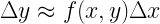
We have that

$y' = \frac{{dy}}{{dx}} = f(x,y) \approx \frac{{\Delta y}}{{\Delta x}}$

where Δy and Δx are along the tangent line as in the figure below.

We thus have

$\Delta y \approx f(x,y)\Delta x$

We can now add Δx to our x and Δy to our y to get to our next point. This gives us the following algorithm.

I: Select a step length Δx.

II: Start at (x₀, y₀) and set n=0

III: Let

$\Delta y = f({x_n},{y_n})\Delta x$

IV: Let

$\begin{gathered} \Delta y = f({x_n},{y_n})\Delta x \hfill \\ {y_{n + 1}} = {y_n} + \Delta y, \hfill \\ {x_{n + 1}} = {x_n} + \Delta x, \hfill \\ n = n + 1 \hfill \\ \end{gathered}$

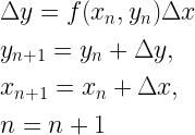
Repeat step IV as many times as necessary.

Let us look at an example. Why not the

$y' - xy = {x^2}$

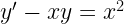
again. This can be rewritten as

$y' = xy + {x^2}$

Say we choose to start at (1, 2) and select Δx=0.1, and say we want an approximate answer for our differential equation at x=2. For our first step, we get

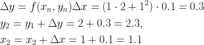
$\begin{gathered}\Delta y = f({x_n},{y_n})\Delta x = (1 \cdot 2 + {1^2}) \cdot 0.1 = 0.3 \hfill \\ {y_2} = {y_1} + \Delta y = 2 + 0.3 = 2.3, \hfill \\ {x_2} = {x_2} + \Delta x = 1 + 0.1 = 1.1 \hfill \\ \end{gathered}$

(We don’t need to explicitly keep track of n, since we do it as we rename our variables anyhow, and if we wrote a program to do this, and if we are not interested in the points along the way, we may just overwrite our old variables).

We can then do this over and over again. This gives us

	Δt=	0.1
n	x	y	Δy
0	1.0	2	0.3
1	1.1	2.3	0.374
2	1.2	2.674	0.46488
3	1.3	3.13888	0.577054
4	1.4	3.715934	0.716231
5	1.5	4.432165	0.889825
6	1.6	5.32199	1.107518
7	1.7	6.429508	1.382016
8	1.8	7.811525	1.730074
9	1.9	9.541599	2.173904
10	2.0	11.71550	2.743101

The above was done in Excel. On another page we found that y should be about 13.96225 for x=2, so we are not particularly close. A smaller step size (Δx) might help though. Below we have a table of step size vs answer.

Δx	N	y	Error
1	1	5	8.962250
0.1	10	11.71550	2.246747
0.01	100	13.69724	0.265014
0.001	1000	13.93526	0.026986

So basically we are moving along the slopes in a slope field as in the figure below. In the graph, the actual solution is shown too.

As you can see the approximate solution gets worse and worse as we get further along our approximate curve. The reason for this is that we use the slope at the starting point of an interval as our slope along the interval, but in actuality, the slope changes over the interval as seen in the enlarged part of the figure below.

The method, called Euler’s step method, is not the best possible, for the above reasons, but it is quite general and is a first step towards learning other, more accurate methods.

Up a level : Differential Equations
Previous page : Simple harmonic motion again – using Taylor series
Next page : Simple harmonic motion –Euler’s step method

Last modified: Dec 28, 2023 @ 16:57