Previous page : On the Bouncing balls program
Next page : Galton Board
Bounces
To start with, to find the position for the next bounce we can set up a system of equations, one equation for the bowl and one for the parabolic path of a ball. This can then be rewritten into a quartic (fourth-degree) equation. This is solved using a method found in Practical Algorithms for Solving the Quartic Equation by David J. Wolters. I used Ferrari’s Method, the modified algorithm, and changed it to be able to give complex roots too.
I calculate the times for the ball to reach the ceiling (if ever) and one of the walls + the bowl, and then I use the shortest time as the time to the next bounce.
As the ball advances, its position is calculated using the time-dependent equation of its path.
The time ticks on with ticks of fixed duration, and as soon as the time passes the time for the next bounce a new trajectory is calculated, with a new start position, and a new initial velocity.
Those values are calculated from the time at the collision, then the ball is moved corresponding to how much is left of the current time slot.
If the calculated time to the next collision is shorter than the remaining time, e.g., if the ball was very close to a corner, then the collision method is recursively called again. This happens very rarely since the ball has to be very close to a corner for a new bounce to happen within the remaining time of the 1 ms time slot.
Direction of the bounces
Here we need a bit of vector algebra.
At the bounce, we have some velocity of the incoming ball, and we need to find the velocity after the bounce. Say the in velocity is v and the out velocity is w. We also need the slope of the bowl at the point of collision. Say that is m. We will also use a vector p, that is parallel with the tangent line of the bowl at the point of reflection.
To simplify the maths, we want the vector p to have the length 1. This gives us that
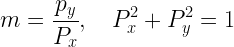
or
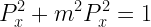
and thus
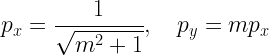

As we can see in the figure the sum of w and v will be parallel with p. We have that

for some scalar, s. This gives us
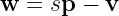
The LHS and RHS of this obviously have the same length, this can give us the idea that squaring both sides could be a good idea. This gives us

The two vectors of w and v have the same length, and p=1, so we get,

or

And finally

This is implemented as the method
|
1 2 3 4 5 6 7 8 |
reflect: function (m, vx, vy) { let px = 1 / Math.sqrt(m ** 2 + 1); let py = px * m; let s = 2 * (vx * px + vy * py); let ux = s * px - vx; let uy = s * py - vy; return [ux, uy]; } |
On the exponential growth of the average distances
If one drops the balls from the centre and with a distance between the balls of a 10-9 pixels, then the following graph shows the log 10 of the average distance between successive balls vs.. time. The distance grows by a factor of about 1.4 per second.

If one instead looks at the log base 10 of the horizontal distance between ball 127 and ball 128, which falls straight down, we can see a virtually perfect fit to a straight line.

In the table below we can see some of the data. We can see the quotients between successive values of x are virtually constant, and that it is the same as the quotients between successive velocities. The latter makes sense given that the time between successive bounces is close to constant as the ball basically just bounces straight up and down, and thus the small shift in horizontal position should be proportional to the velocity – that is proportional to the shift in position that … and so on. That means that, for this kind of almost straight up and down motion whatever initial quotient between initial velocities we have should just remain, as can be observed.
| t [s] | x [pixels] | v [px/ms] | xn+1/xn | vn+1/xn | x/v |
| 3.26 | -1.00E-09 | 0.00E+00 | |||
| 9.77 | 1.22E-08 | 2.03E-12 | -12.23 | 6020 | |
| 16.28 | -1.36E-07 | -2.28E-11 | -11.15 | -11.23 | 5976 |
| 22.78 | 1.52E-06 | 2.54E-10 | -11.14 | -11.14 | 5976 |
| 29.29 | -1.69E-05 | -2.83E-09 | -11.14 | -11.14 | 5976 |
| 35.80 | 1.89E-04 | 3.16E-08 | -11.14 | -11.14 | 5976 |
| 42.32 | -2.10E-03 | -3.52E-07 | -11.14 | -11.14 | 5976 |
| 48.82 | 2.34E-02 | 3.92E-06 | -11.14 | -11.14 | 5976 |
| 55.34 | -2.61E-01 | -4.37E-05 | -11.14 | -11.14 | 5976 |
| 61.85 | 2.91E+00 | 4.87E-04 | -11.14 | -11.14 | 5976 |
How about the last quotient, between x and v? The time for one bounce, up and down is about 6512 ms. If we now divide how many times longer one movement took than the last (11.14 times longer), which is also how many times longer x is, by the speed, which is the total distance 11.14 (current)+1 (previous) we get 6512·11.14/12.14 = 5976….
Previous page : On the Bouncing balls program
Next page : Galton Board